
Among the essential performance metrics used in the process of backtesting trading strategies the Sharpe ratio is one of the most widely used. It helps traders assess the risk-adjusted returns of a strategy. This article will provide an in-depth exploration of the Sharpe ratio, its significance, calculation, and interpretation, as well as guidance on what Sharpe ratio values are considered good or acceptable in trading context.
Formula of the Sharpe Ratio
The Sharpe ratio, developed by Nobel laureate William F. Sharpe in 1966, is a measure that helps traders and investors evaluate the return of an investment relative to its risk. More specifically, it shows how much excess return an investment generates for each unit of risk taken. The formula for the Sharpe ratio is as follows:
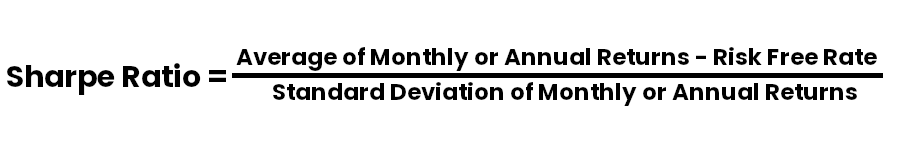
Here, the average of monthly or anual returns refer to the returns generated by the trading strategy, while the risk-free rate is the return of a theoretically risk-free investment, such as government bonds. The standard deviation of returns measures the volatility of the strategy, which serves as a proxy for risk. Although the Sharpe ratio is widely applicable across different investment instruments, this article specifically focuses on its application within the trading context.
Importance of the Sharpe Ratio in Backtesting
Backtesting involves simulating a trading strategy on historical data to assess its potential performance. While absolute returns are a key focus, they don’t always provide a full picture of the strategy’s efficiency. This is where the Sharpe ratio plays its role, as it normalizes returns relative to the risk taken, offering a clearer perspective on the strategy’s true value.
High returns may seem appealing, but if they come with significant volatility, they could indicate excessive risk. The Sharpe ratio adjusts for this, highlighting whether the returns are truly worth the risk taken. It offers a way to gauge the risk-adjusted performance of a strategy, helping traders avoid being misled by high, yet unstable returns.
Additionally, the Sharpe ratio allows for easy comparison across multiple strategies. Even if one strategy delivers lower absolute returns, a higher ratio could make it a better option than a high-return strategy with much higher risk. By focusing on risk-adjusted performance, the Sharpe ratio offers a more balanced view when comparing different trading strategies.
Components of the Sharpe Ratio
To understand how the Sharpe ratio functions in a backtesting environment, it’s crucial to break down each component:
- Return: This is the return generated by your trading strategy. Returns are often calculated on a monthly or annual basis, depending on the time frame and strategy being tested.
- Risk-Free Rate: The risk-free rate represents a return on a riskless investment. It’s common to use the yield on short-term government bonds (3 Month T-Bills) as a benchmark for this rate. Over short time frames, the risk-free rate can be close to zero, but over long periods, this rate can have big impact, especially if returns are only marginally higher than risk-free alternatives.
- Standard Deviation (Volatility): The standard deviation of returns measures the strategy’s volatility. It tells you how much returns fluctuate over time. Strategies that exhibit consistent returns will have lower volatility and, thus, a higher Sharpe ratio, assuming returns exceed the risk-free rate.
Calculating the Sharpe Ratio in Excel Spreadsheets
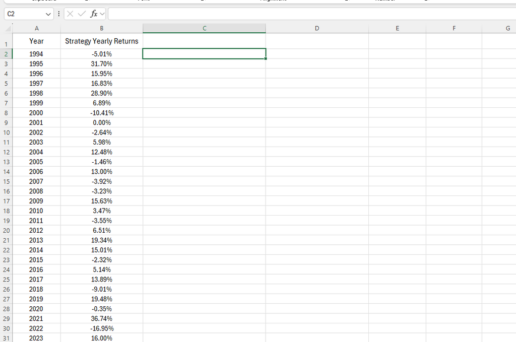
Let’s assume we have a list of yearly returns from a trading strategy.
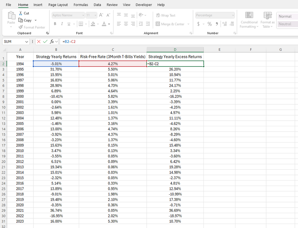
Step 1: Adjust for the Risk-Free Rate
Start by subtracting the risk-free rate from the strategy’s yearly returns. As shown in the spreadsheet, the risk-free rate can vary over time as T-Bill yields fluctuate. For simplicity, many traders use a constant average risk-free rate.
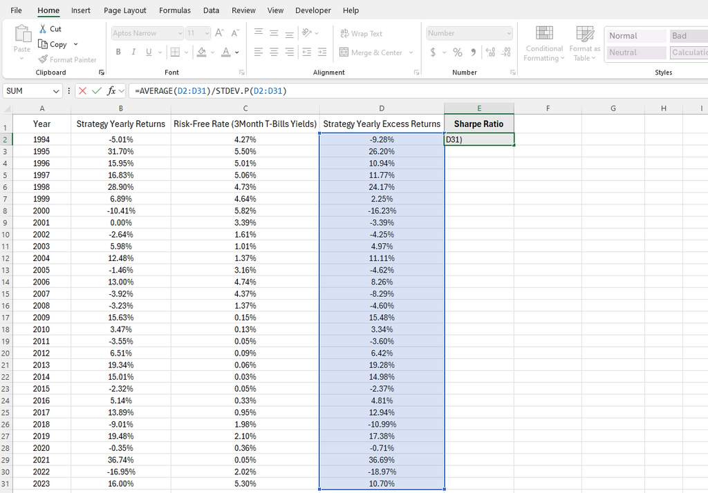
Step 2: Calculate the Sharpe Ratio
Next, calculate the Sharpe ratio by dividing the average of the excess returns by the standard deviation of these returns.
Download this Excel spreadsheet. If you need a more detailed spreadsheet with formulas for calculating monthly and annual returns, as well as 18 performance metrics for testing trading strategies, consider our backtesting spreadsheets.
Interpretation of the Sharpe Ratio
The Sharpe ratio offers a convenient measure of risk-adjusted return, combining both the profitability and riskiness of a strategy into a single number. However, the interpretation of this metric can vary depending on the context and time horizon.
Generally, a Sharpe ratio of around 1.0 is considered good. It indicates that the strategy produces returns roughly proportional to the amount of risk taken, which makes it worth considering, especially over shorter timeframes.
Values above 2.0 is often considered excellent, indicating that the strategy is generating substantial excess returns for the level of risk assumed. However, it’s important to recognize that sustaining such a high ratio over long periods is rare, as market conditions change, and systematic inefficiencies are exploited. Robert Carver’s analysis of hedge funds highlights that very few can maintain a Sharpe ratio above 1.0 consistently over several years. This suggests that traders should be cautious in interpreting very high Sharpe ratios, as they could point to short-term outperformance that might not persist in live markets.
Caution on High Sharpe Ratios
A Sharpe ratio above 3.0 might seem like the “holy grail” of trading, but in many cases, it could be a sign of overfitting in backtesting. High Sharpe ratios can result from excessive optimization of parameters to historical data, which often leads to performance that does not hold up in live trading. Therefore, traders should be skeptical of strategies that produce such extreme values and focus on ensuring robustness rather than chasing exceptional backtest results.
Understanding High Sharpe Ratios in Backtesting
When running a backtest with in-sample data, it’s not uncommon to encounter a Sharpe ratio (SR) of 3 or even higher. It can be expected in such cases because the strategy is optimized for the historical data it was trained on. In this phase, you’re primarily concerned with making sure the strategy captures key market patterns and refining parameters, so there is no immediate reason to worry about overfitting based on the SR alone.
However, the real test comes when you move to out-of-sample validation. At this stage, you’ll likely see a more realistic, lower SR, perhaps around 1.0 or even lower. This drop is normal and should not be a source of frustration. In real-world trading, even a SR below 1.0 can still result in profitable, sustainable strategies. In fact, many traders see SR in the range of 0.3 to 0.5, and this is perfectly acceptable for live trading. While these values might seem low compared to backtesting results, they are more reflective of actual market conditions, including transaction costs, slippage, and periods of higher volatility.
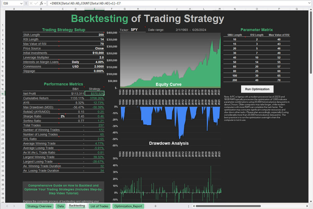
Free Backtesting Spreadsheet
Limitations
While SR is a valuable tool for assessing risk-adjusted performance, it has its limitations.
- Assumes Normal Distribution of Returns: SR assumes that returns are normally distributed, but financial markets often exhibit fat tails and skewness. Extreme events, like market crashes, can disproportionately affect SR because it doesn’t account for the higher likelihood of significant deviations from the mean, such as in times of crisis. In such scenarios, a metric like RoMaD (Return over Maximum Drawdown) can be more effective. RoMaD evaluates returns relative to the worst observed loss (maximum drawdown), providing different way to gauge risk for strategies exposed to rare but extreme losses.
- Ignores Time Dependency: SR does not account for the timing of returns. A strategy may generate high returns over a short period and then underperform for an extended time, skewing SR.
- Volatility as a Risk Measure: SR uses volatility as the sole measure of risk. However, not all volatility is negative. For instance, upward volatility (positive returns) is often desirable. For example, the Sortino ratio address this by focusing on downside risk.
Sharpe Ratio vs. Profitability: Same Ratio, Different Outcomes
Two strategies with identical SR can have drastically different profitability profiles. For example, consider Strategy A with a 10% return and 10% volatility and Strategy B with a 20% return and 20% volatility. Both strategies yield a SR of 1, suggesting they have the same risk-adjusted return. However, the absolute return of Strategy B is twice that of Strategy A. A similar effect occurs when leverage is used, as it increases both the return and volatility proportionally.
Even though the risk-adjusted performance is the same, Strategy B is more profitable in absolute terms. This highlights an important limitation of SR: it does not account for the magnitude of returns, only their proportion to risk (volatility). In real-world trading, higher returns—even with proportionally higher risk—can still be more desirable.
For instance, institutional investors might prefer a strategy with a lower absolute return but more stability, while an individual trader might prioritize strategies that yield higher profits, even if they carry more risk. In practice, traders should not rely solely on SR to choose between strategies but also consider their specific goals, risk tolerance, and capital requirements.
Improving the Sharpe Ratio Through Diversification
If your backtested SR is lower than desired, enhancing it through diversification is a highly effective approach. By combining multiple trading strategies that are uncorrelated, you can mitigate overall portfolio risk and achieve more stable returns. This approach ensures that when one strategy underperforms, another may still generate positive returns, which can lead to a more consistent risk-adjusted performance.
Additionally, diversifying across different asset classes—such as stocks, bonds, and currencies—can help reduce the impact of market downturns. Different asset classes often react differently to economic events, leading to lower overall volatility. Incorporating a mix of trading styles, such as trend-following and mean-reversion, can also enhance resilience in varying market conditions.
Final Thoughts
SR is an indispensable tool for evaluating the risk-adjusted performance of a trading strategy during backtesting. It provides a clear and concise measure of whether a strategy’s returns are worth the risk taken. However, like all metrics, it has its limitations and should be used in conjunction with other performance metrics.
When applied thoughtfully, SR can significantly enhance your strategy development process, enabling you to identify strategies with sustainable and consistent returns. Just remember, the ultimate goal is not just to maximize SR but to find a strategy that passes the test of time and delivers consistent performance in live trading.
Share on Social Media:
FAQ
What Sharpe ratio is good?
A Sharpe ratio about 1.0 is generally considered good. It indicates that the strategy generates returns proportional to the risk taken, which is often a sign of a well-balanced strategy.
Is a Sharpe ratio below 1 bad?
A Sharpe ratio (SR) below 1.0 is not necessarily bad, but it suggests that the returns are not much higher than the risk. Many profitable strategies may have SRs between 0.5 and 1.0, especially in live trading, where market conditions are unpredictable.
What Sharpe ratio is considered bad?
A Sharpe ratio below 0 is definitely bad. It indicates that the strategy is generating negative risk-adjusted returns, meaning you would have been better off holding a risk-free investment instead of trading.
Is a Sharpe ratio of 0.5 good?
A Sharpe ratio of 0.5 is acceptable in some cases, especially for strategies exposed to high volatility or in live trading environments. While it’s not ideal, strategies with this ratio can still be profitable with proper risk management.

Leave a Reply